

RTN-132
Unrecognized blends in LSST DP2 from the comparison with Euclid and HST#
Abstract#
Unrecognized blends, objects that correspond to several truth sources, are a known issue in LSST data and a significant source of photometric error. In this technote, we identify unrecognized blends in the LSST Data Preview 2 dataset (DP2) by comparing it to high-resolution, space-based observations from Euclid Q1 and the Hubble Space Telescope (HST) in the Extended Chandra Deep Field South (ECDFS). By matching sources detected in the LSST data with those from the space telescopes, first by position and then by the overlap of their observed shapes, we quantify the fraction of LSST objects that are unrecognized blends, i.e. blended in LSST but resolved in the space-based data. We find that up to 22% of sources in DP2 are unrecognized blends when compared to Euclid Q1 data for \(23 < i < 24\). When compared to HST data, the fraction of unrecognized blends reaches up to 40% for the same magnitude range. Since this binary classification depends strongly on the depth of the reference survey, we then use the blending entropy \(S_\text{b}\), a continuous metric that combines shape overlap with photometry, to quantify how ambiguous the galaxy association of each unrecognized blend is. This metric gives broadly consistent results for Euclid and HST down to the magnitude where Euclid, the shallower reference survey, becomes incomplete. This reconciles the two comparisons: at \(i \simeq 23.5\), \(19\%\) of DP2 objects have \(S_\text{b} > 0.2\) when compared to Euclid and \(16\%\) when compared to HST. These fractions are expected to decrease with the better image quality of LSST Data Release 1, and they are directly relevant to the calibration of blending effects in weak-lensing analyses.
Introduction#
Blending, where multiple sources visually overlap on the sky, is expected to be a significant source of uncertainty for Stage-IV ground-based surveys like LSST [Melchior et al., 2021]. Blended sources can often be identified and deblended. Unrecognized blends are a distinct case: objects that are detected as a single source in the survey data but that correspond to several distinct truth sources. Because the pipeline treats them as isolated objects, their properties (fluxes, colors, shapes) cannot be measured accurately or independently, and they are not flagged as blends. One way to study blending is to compare data from different telescopes with different resolutions and depths. Space-based observations have a higher angular resolution than ground-based ones because they are not affected by atmospheric turbulence, which broadens the point spread function (PSF), so blends unrecognized in ground-based images may be resolved in space-based images.
In this note, we use Euclid Q1 and HST imaging of the Extended Chandra Deep Field South to measure the fraction of unrecognized blends in the LSST DP2 datasets as a function of magnitude, and we quantify how ambiguous these blends are with the blending entropy [Ramel et al., 2026], a continuous metric that, unlike a binary match, is largely insensitive to the depth of the reference survey.
Data#
The Extended Chandra Deep Field South (ECDFS) is a deep survey field that has been observed by many telescopes at different wavelengths due to its low Galactic extinction [Lehmer et al., 2005]. In this note, we use imaging of the ECDFS from three facilities.
Rubin LSST: Rubin Observatory’s Data Previews are early releases that precede LSST Data Release 1. Data Preview 1 (DP1) [Vera C. Rubin Observatory Team, 2026] is based on commissioning observations from the LSST Commissioning Camera (LSSTCam’s smaller predecessor, ComCam) and includes ECDFS among its fields. Data Preview 2 (DP2) [Vera C. Rubin Observatory Team, 2026] is the first preview based entirely on data from the full LSST Science Camera (LSSTCam) and also covers the ECDFS. Both have a pixel scale of 0.2 arcsec/pixel. To access the LSST DP2 data, we use the Rubin Science Platform (RSP) and the
butlerAPI. The following parameters are used to specify the repository, collection, skymap, and catalog:
repo='dp2_prep'
collection = 'LSSTCam/runs/DRP/DP2/v30_0_8/DM-55060/stage3'
skymap = 'lsst_cells_v2'
butler_cat = 'object'
Euclid Q1: The Euclid Quick Data Release 1 (Q1) [Euclid Collaboration et al., 2026] is an early release of Euclid imaging and spectroscopy over ~63 deg² in three Euclid Deep Fields, one of which (Euclid Deep Field Fornax) contains the ECDFS. We use the VIS optical imaging, which has a pixel scale of 0.1 arcsec/pixel. We use the final MER (MERge) catalog from Euclid Q1, which merges the VIS and NISP space-based imaging with external ground-based data to produce the combined multi-band source catalog.
HST: The Hubble Space Telescope also imaged the ECDFS [Illingworth et al., 2016], providing high-resolution imaging with a pixel scale of 0.06 arcsec/pixel. We use the Hubble Legacy Fields (HLF) GOODS-South source catalog, which is a high-level science product derived from archival HST imaging.
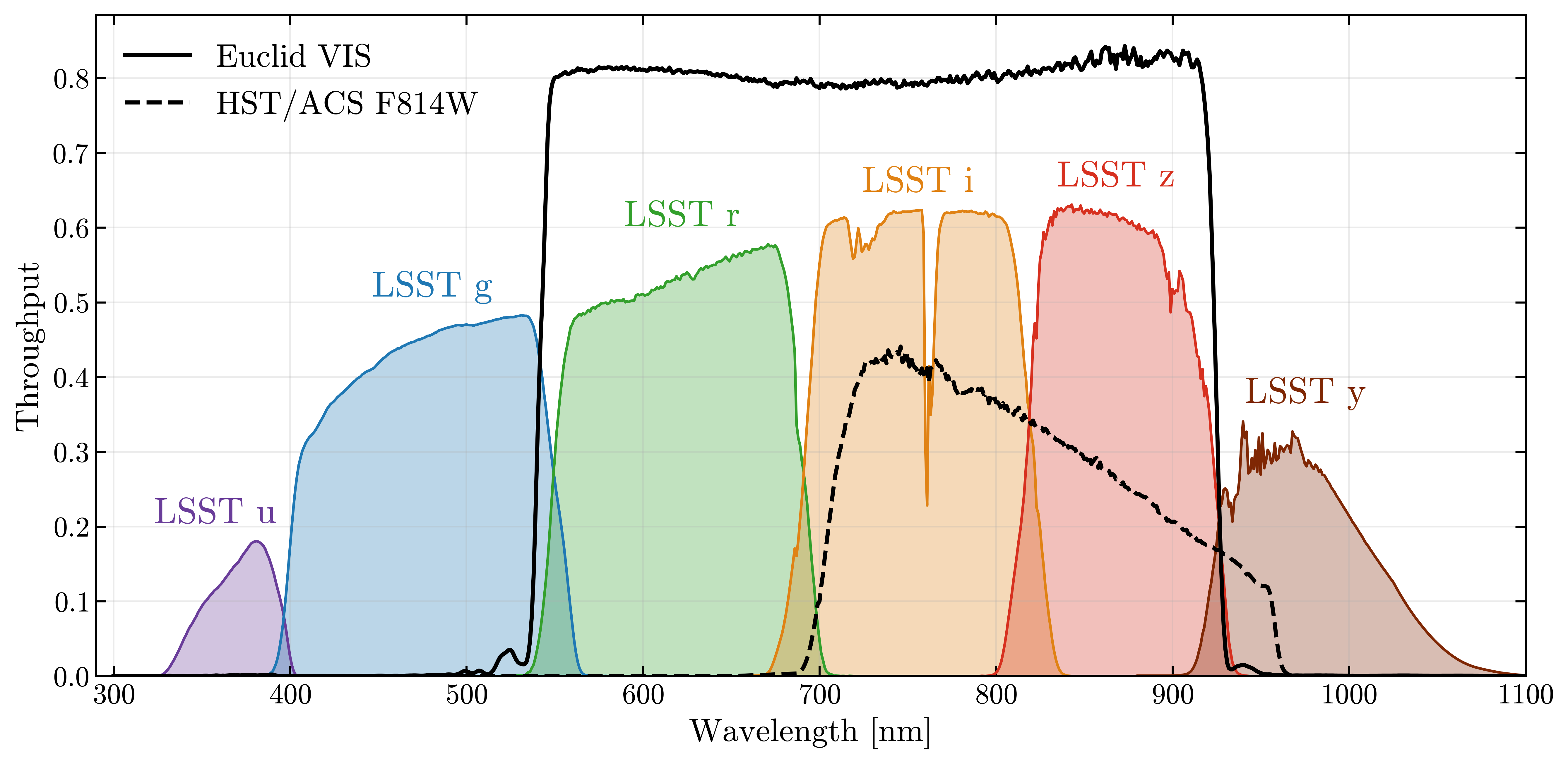
Fig. 1 Bandpasses of the LSST, Euclid and HST filters used in this study.#
As shown in Fig. 1, the LSST, Euclid and HST filters used in this study cover overlapping wavelength ranges. The LSST \(riz\) bands are the closest to the Euclid VIS band, and the LSST \(i\) band is the closest to the HST F814W band.
The datasets also overlap spatially in the ECDFS, as shown in Fig. 2. The LSST DP2 and Euclid footprints cover the entire ECDFS field, while the HST footprint covers a smaller area within the ECDFS. Some areas of the LSST DP2 data are covered by only a single visit, which can lead to shallower detections and artifacts. To avoid these effects we restrict the LSST data to a circular region of radius 2.1 degrees centered on the coordinates RA=53.05, Dec=-28.15 degrees, which is free of single visits and has a homogeneous depth.
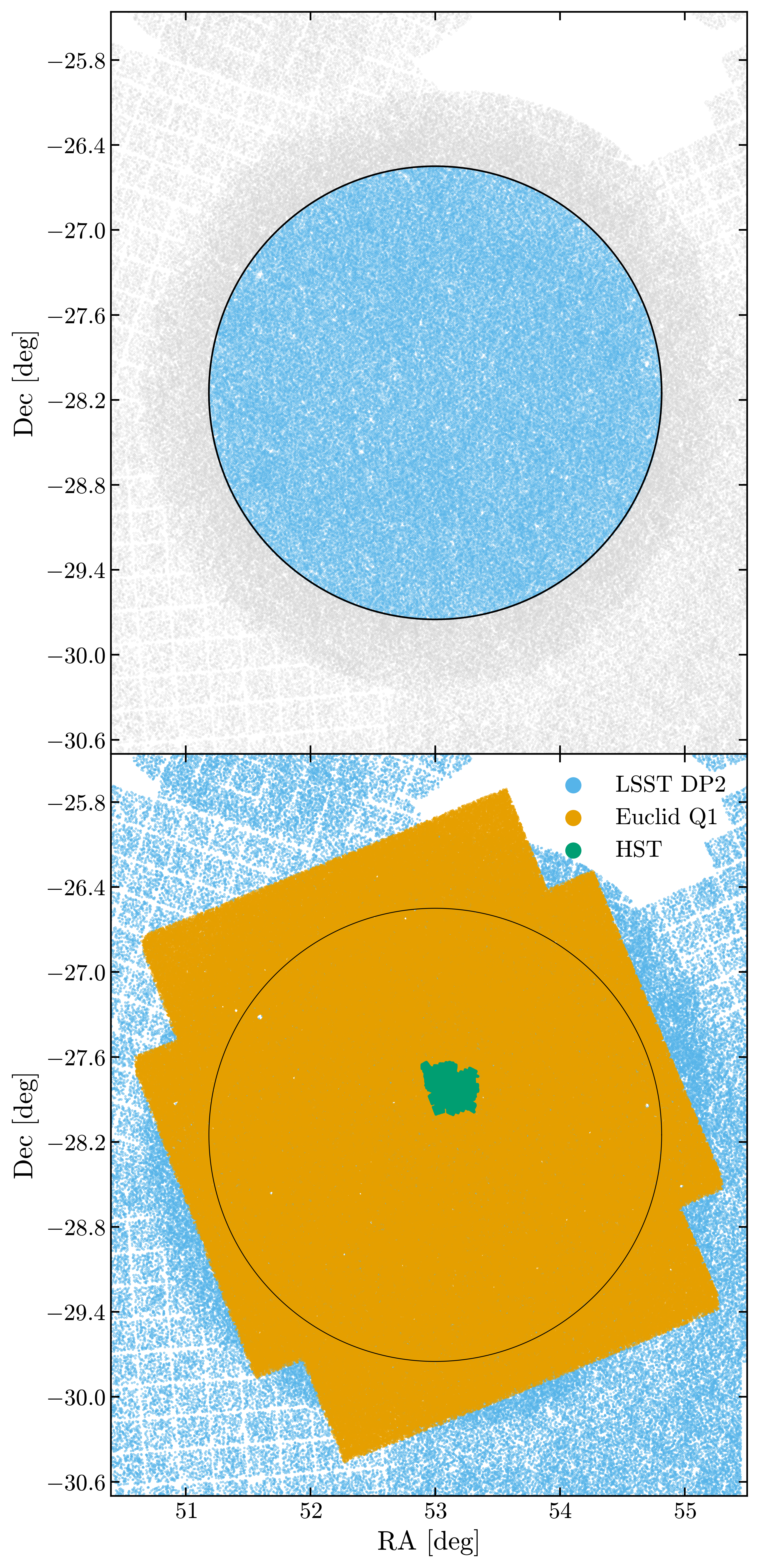
Fig. 2 Top: One tenth of the detected galaxies in the ECDFS observed by LSST. The blue region corresponds to our region of study, chosen to avoid single-visit effects (shallower detections and artifacts). The grey region is discarded due to the presence of single visits. The circle separating the two regions has a radius of 2.1 degrees and is centered on the coordinates RA=53.05, Dec=-28.15 degrees. Bottom: One tenth of the detected galaxies in the ECDFS observed by LSST, Euclid and HST.#
The Euclid ECDFS footprint has an area of 15.5 deg2 and contains 5,328,489 galaxies detected in the VIS band and 2,416,305 objects detected in the LSST DP2 dataset.
The HST ECDFS footprint has an area of 0.18 deg2 and contains 165,776 galaxies detected in the F814W band and 33,240 objects detected in the LSST DP2 dataset.
In the following sections, we will refer to sources detected in the LSST DP datasets as objects and to sources detected in the Euclid and HST datasets as (reference) galaxies. We call unrecognized blends the objects that are matched with more than one reference galaxy. Unless stated otherwise, all plots are for the LSST DP2 dataset.
Methods#
The pipeline described below is available at https://github.com/LSSTDESC/copaings.
Matching LSST DP catalogs with Euclid and HST#
We match the sources detected in the LSST DP datasets with those from Euclid and HST using a two-step process:
Friends-of-friends (FoF) catalog matching [Mao et al., 2021]: pairs of “friends” within a specified linking length are connected iteratively and transitively, and their associated groups are merged. It starts with each object as its own group, then recursively merges groups if any member of one group is within the linking length of any member of another. The choice of linking length defines the scale of the resulting structures. We chose a linking length of 2 arcsec to make coarse groups, in which all elements are initially connected to each other. This length is larger than the typical size of the PSF-convolved ellipses, and we checked that larger linking lengths have a negligible impact on our results.
Ellipse Overlap Test (EOT): For each element (either an object or a galaxy) in each group, we define an elliptical footprint computed from the semi-major and semi-minor axes and the position angle of the detection. For that footprint, we also account for the effect of the local LSST PSF by convolving the ellipse with it. Starting from densely connected FoF groups, we perform a geometric test to determine whether the ellipses of each pair of elements overlap. If there is no overlap between two elements, we remove their link. If non-overlapping subsets are found, we split the group into subgroups until all elements in each group are connected through overlapping ellipses. We discard groups made of a single element (object or galaxy).
Adding the EOT step after the FoF matching makes our matching independent of the linking length choice, provided the linking length is large enough to capture all overlapping elements. The result of this matching is a set of groups where each group contains one or more objects and one or more galaxies. Elements within a group overlap, at least transitively. From this matching, we compute the number of objects and galaxies per group, as shown in Fig. 3.
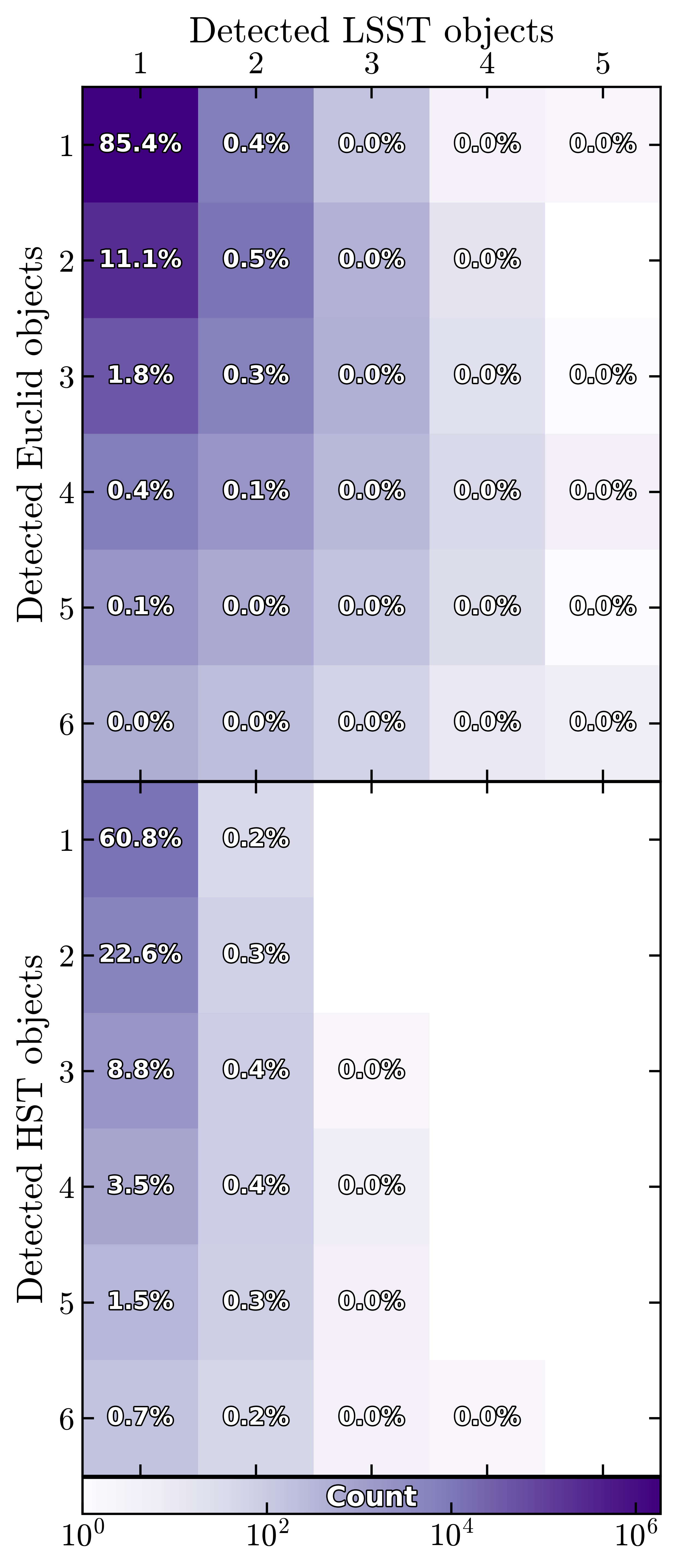
Fig. 3 Results of the LSST–Euclid and LSST–HST cross-matching with the FoF+EOT method. Each bin of the 2D histogram counts the groups with a given number of objects (LSST detections, in columns) and galaxies (Euclid detections, top, or HST detections, bottom, in rows). The colorbar indicates the number of groups in each bin.#
By construction, an unrecognized blend belongs to a group with at least two galaxies. Groups with more galaxies than objects, in the lower-left part of Fig. 3, are those in which LSST detects fewer sources than the reference survey.
Blending entropy#
The matching described above provides a binary classification of LSST objects, which depends strongly on the depth of the reference survey: a deeper survey detects more faint companions and therefore finds more unrecognized blends, even when these companions contribute little to the flux of the LSST object. To obtain a blending metric that is continuous and largely insensitive to the depth of the reference survey, we assign to each object detected in the LSST DP a blending entropy value [Ramel et al., 2026] that quantifies how ambiguous its galaxy association is. The blending entropy for a given wavelength band is defined as:
\(p_\text{og}\) is the matching probability of object \(o\) with galaxy \(g\), given by the intersection-over-union \(\left\langle \text{o},\text{g} \right\rangle\) of the two ellipses — the area they share divided by the area they cover together, ranging from 0 (disjoint) to 1 (identical) — weighted by an exponential factor in their magnitude difference. The probabilities are normalized per object so that \(\sum_{\text{g}\in\text{gal}}p_\text{og} = 1\). Systems with one object and one galaxy have a matching probability of 1 and a blending entropy of 0. The blending entropy ranges from 0, meaning no ambiguity, to \(\ln N\), meaning maximum ambiguity, where \(N\) is the number of galaxies in the overlapping group. Because each galaxy is weighted in \(p_\text{og}\) by its magnitude difference with the object, faint companions contribute little to the blending entropy, as long as the reference survey is deep enough to detect the galaxies that dominate the flux of the object.
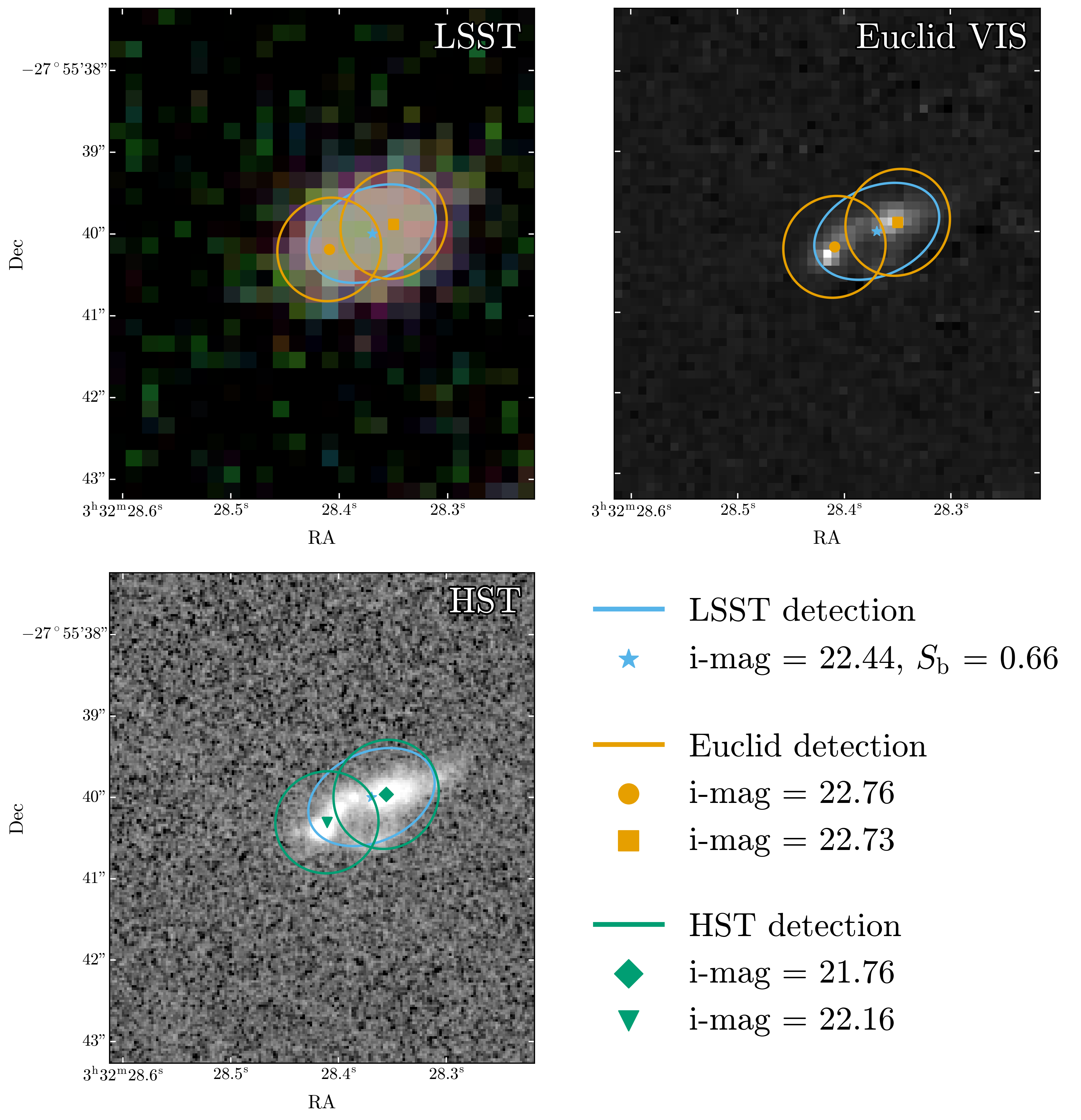
Fig. 4 Example of a high-\(S_\text{b}\) blend. Top: LSST DP2 cutout with \(i,r,g\) bands corresponding to red, green and blue respectively. Middle: Euclid VIS. Bottom: HST F814W. The object from the LSST detection is represented by the blue ellipse; galaxies from the Euclid and HST detections are represented by the orange and green ellipses, respectively. The Euclid and HST ellipses were convolved with the LSST PSF to account for the difference in resolution.#
Fig. 4 shows an example of a high-blending-entropy system with one object and two galaxies. The object overlaps with both galaxies and has a similar magnitude to both of them, making its association with either of the two galaxies ambiguous. The blending entropy for this object is \(S_\text{b} = 0.66\).
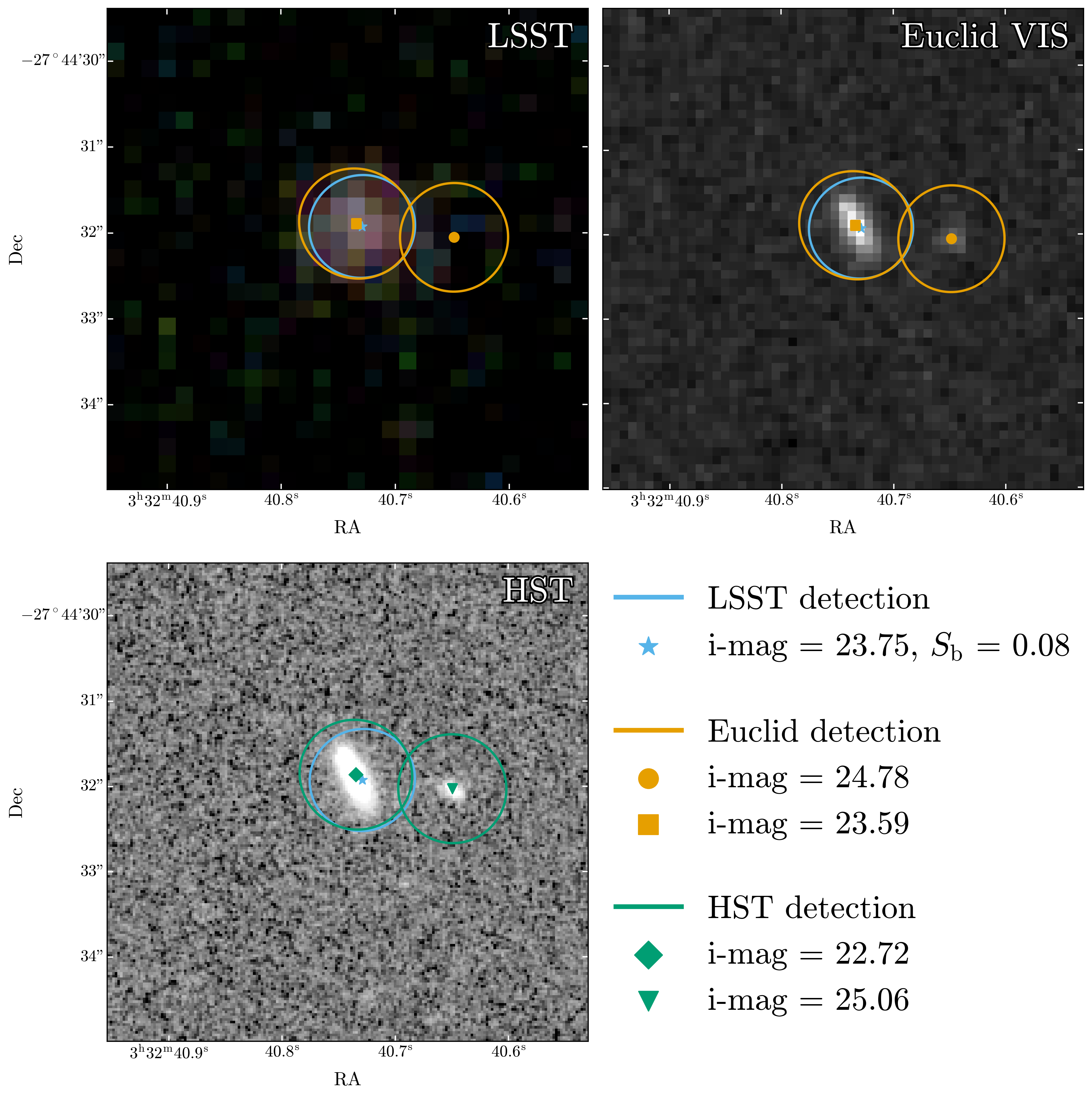
Fig. 5 Example of a low-\(S_\text{b}\) blend. Top: LSST DP2 cutout with \(i,r,g\) bands corresponding to red, green and blue respectively. Middle: Euclid VIS. Bottom: HST F814W. The object from the LSST detection is represented by the blue ellipse; galaxies from the Euclid and HST detections are represented by the orange and green ellipses, respectively. The Euclid and HST ellipses were convolved with the LSST PSF to account for the difference in resolution.#
Conversely, Fig. 5 shows an example of a low-blending-entropy system with one object and two galaxies. One of the Euclid detections overlaps almost entirely with the LSST detection, while the other overlaps only partially and is more than one magnitude fainter. The LSST detection is therefore unambiguously matched with the brighter Euclid detection. The blending entropy for this object is \(S_\text{b} = 0.08\).
The blending entropy compares the magnitude \(m_\text{o}\) of each LSST object with the magnitudes \(m_\text{g}\) of the reference galaxies, which requires both to be measured in the same band. Since Euclid and HST observe in the VIS and F814W bands, which have no exact LSST counterpart (Fig. 1), we predict for each LSST object its VIS or F814W magnitude from its LSST photometry, using the closest LSST bands: \(griz\) for Euclid and \(i\) for HST. The relation between the LSST magnitudes of an object and the measured VIS or F814W magnitude of its reference galaxy is fitted on one-to-one systems only, where both measurements refer to the same galaxy and the photometry is cleanest. This relation is then applied to every object in the LSST DP datasets, and the predicted magnitude is used as \(m_\text{o}\) in the definition of \(S_\text{b}\).
For Euclid, the predicted VIS magnitude depends on the \(r\)-band magnitude and on the \(g-r\), \(r-i\) and \(i-z\) colors:
We define \(r_{\text{term}}\) as a piecewise linear function of \(r\):
If \(r \leq 22\): \(r_{\text{term}} = a_0^{\text{low}} + c_r^{\text{low}} \cdot r\)
If \(r > 22\): \(\,r_{\text{term}} = a_0^{\text{high}} + c_r^{\text{high}} \cdot r\) where we define \(a_0^{\text{high}} = a_0^{\text{low}} + (c_r^{\text{low}} - c_r^{\text{high}}) \cdot 22\) to ensure continuity at \(r = 22\).
For HST, the predicted F814W magnitude is a linear function of the \(i\)-band magnitude: \(\text{F814W}_{\text{fit}} = c_0 + c_{i} \cdot i\)
The fitted coefficients are given in Coefficients of the magnitude fits.
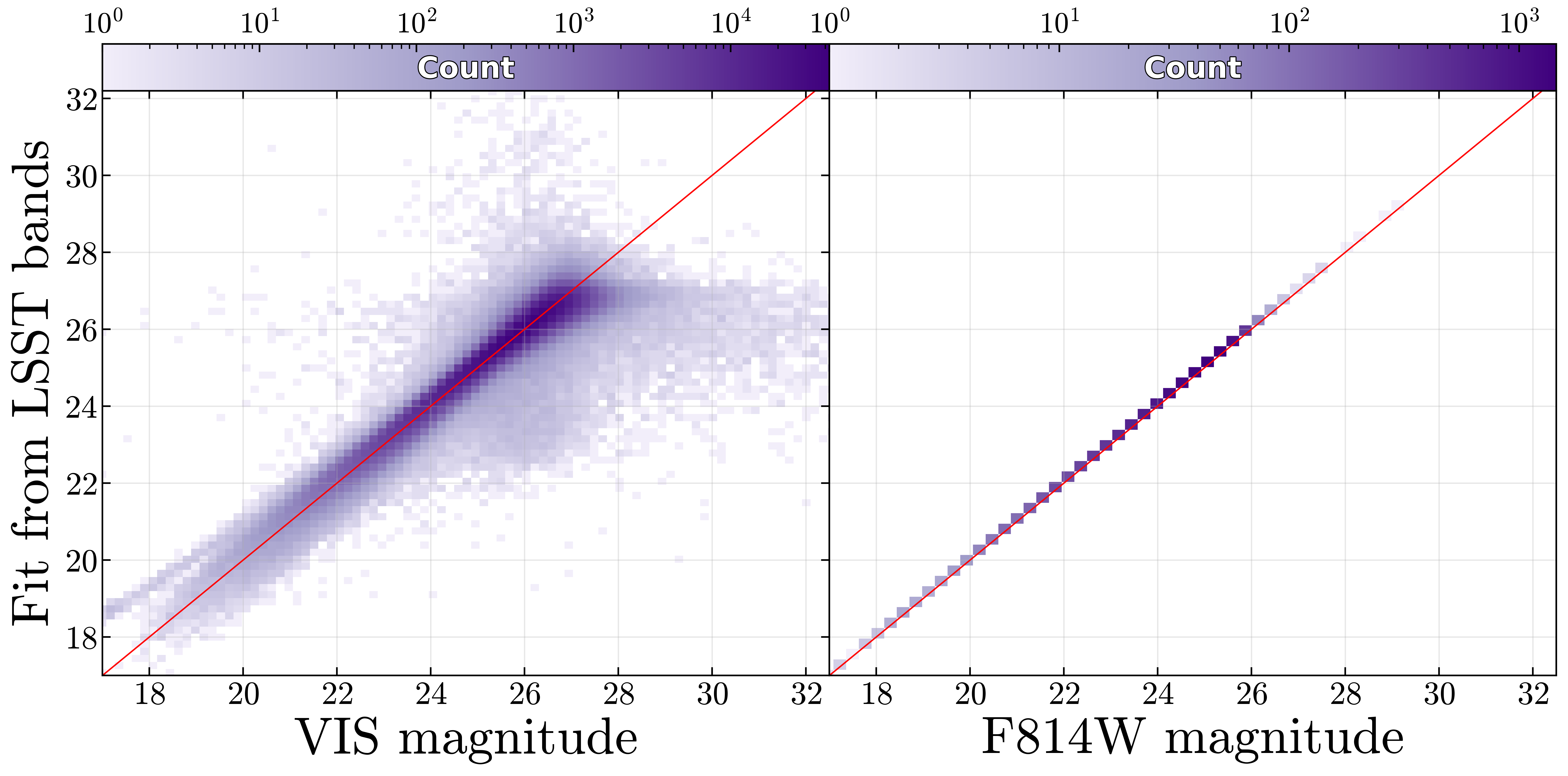
Fig. 6 Verification of the VIS magnitude and F814W magnitude fits. Left: The x-axis is the measured VIS magnitude from Euclid and the y-axis is the predicted VIS magnitude from the LSST DP2 photometry. Right: The x-axis is the measured F814W magnitude from HST and the y-axis is the predicted F814W magnitude from the LSST DP2 photometry. The colorbar indicates the number of objects in each bin. The red line shows \(x=y\).#
Fig. 6 shows that the magnitudes predicted from the LSST DP2 photometry reproduce the measured space-based magnitudes, with a median absolute deviation of about 0.2 mag for both VIS and F814W. For each object in the LSST DP datasets, we can therefore compute the blending entropy with Euclid as the reference, using the VIS magnitude predicted from its \(griz\) photometry, or with HST, using the F814W magnitude predicted from its \(i\)-band photometry.
Results#
Integrated over all magnitudes, 13.8% of LSST DP2 objects are unrecognized blends when compared to Euclid and 38.7% when compared to HST (Fig. 3). As expected from the differences in depth and resolution between the two reference surveys, these fractions differ by almost a factor of three. We now examine how they depend on magnitude and use the blending entropy to determine how ambiguous these blends are.
To do so, we use the blending entropy computed for each LSST DP2 object. Objects with \(S_\text{b} > 0\) are matched with more than one galaxy and are therefore unrecognized blends, while objects with \(S_\text{b} = 0\) are matched with a single galaxy. Among unrecognized blends, we call ambiguous blends those with \(S_\text{b} > 0.2\), i.e. whose galaxy association is ambiguous; see Ramel et al. (2026) for a detailed justification of this threshold. Fig. 7 shows the fractions of both populations as a function of LSST \(i\)-band magnitude.
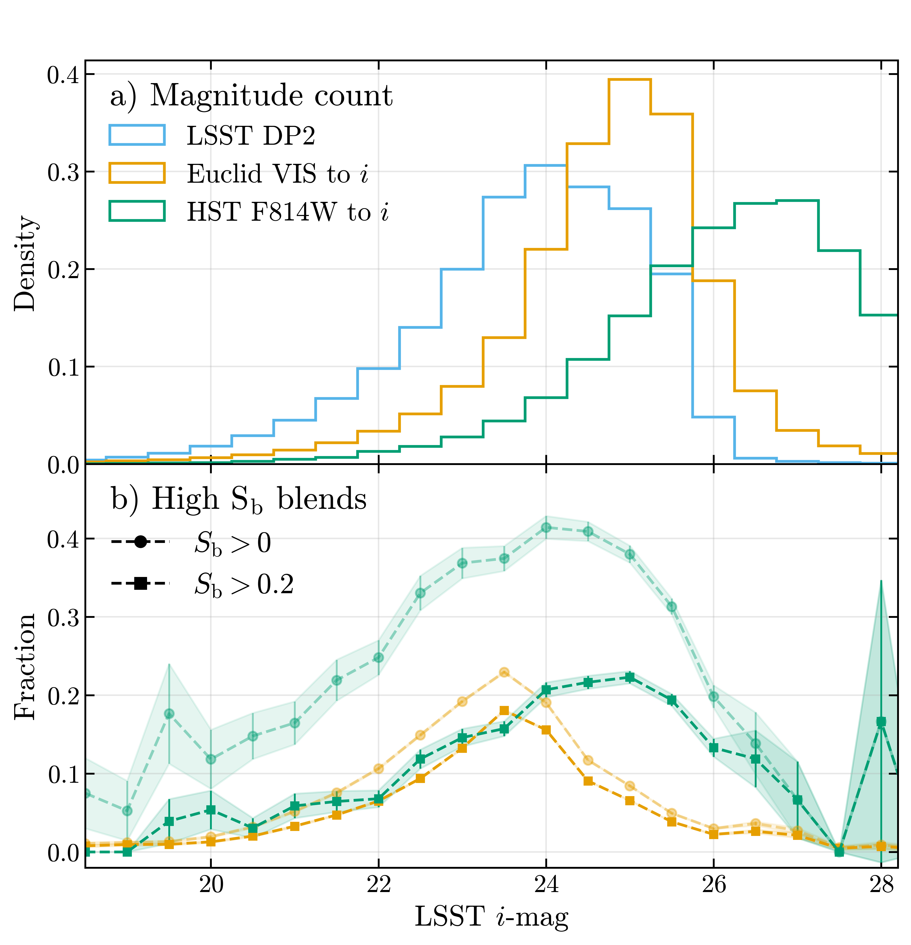
Fig. 7 a) Distribution of detection magnitudes for LSST (blue), Euclid (orange) and HST (green) in ECDFS. Since the observation bands of these telescopes do not cover the same wavelength ranges, the Euclid VIS and HST F814W magnitudes are converted to the LSST \(i\) band with a dedicated fit, used only for this panel and distinct from the fits described in the Methods section. b) Fraction of LSST DP2 objects with \(S_\text{b} > 0\) (circles, unrecognized blends) and \(S_\text{b} > 0.2\) (squares, ambiguous blends), with either Euclid or HST as reference space-based data.#
Fig. 7-a) shows the magnitude distribution for each survey. The HST observations are much deeper than both LSST and Euclid. Fig. 7-b) shows the fraction of unrecognized blends (\(S_\text{b} > 0\)) and the fraction of ambiguous blends (\(S_\text{b} > 0.2\)) as a function of magnitude. The fraction of unrecognized blends is higher for HST than for Euclid, because HST has a better resolution and a greater depth. Many of the additional HST blends consist of a bright galaxy and a much fainter one that Euclid does not detect. For both reference surveys, the fraction of unrecognized blends increases with magnitude, since fainter objects are more likely to be blended. This trend breaks down at \(i \simeq 23.5\) with Euclid as the reference; we interpret this as a depth effect: for fainter LSST objects, the fainter galaxy of the blend increasingly falls below the Euclid detection limit. The fraction of unrecognized blends exceeds 20% for Euclid, which is consistent with the results reported by Adari and von der Linden (2025) and Troxel et al. (2023).
After applying the \(S_\text{b} > 0.2\) cut, the fractions of ambiguous blends obtained with the two reference surveys agree up to \(i \simeq 23.5\), where 19% of DP2 objects are ambiguous blends with Euclid as the reference and 16% with HST. The difference between the two \(S_\text{b} > 0\) curves at brighter magnitudes therefore comes from faint galaxies detected by HST but not by Euclid: the corresponding blends are not ambiguous, since the LSST detection is unambiguously associated with the brighter galaxy of the blend. Perfect agreement between the two references is not expected: the fractions are computed over different footprints, and the HST footprint covers only 0.18 deg2, about 85 times less than the Euclid one, so that the HST fractions are subject to significant sample variance.
In summary, the fraction of unrecognized blends in DP2 depends strongly on the depth and resolution of the reference survey, from 13.8% with Euclid to 38.7% with HST, but most of this difference comes from faint companions that do not make the galaxy association ambiguous. The fraction of ambiguous blends is, in contrast, robust to the choice of reference survey down to the Euclid depth limit, with about one in six DP2 objects being an ambiguous blend at \(i \simeq 23.5\).
Discussion#
In this technote, we matched LSST DP2 objects to Euclid Q1 and HST galaxies in the ECDFS with a FoF + EOT procedure and found that unrecognized blends make up 13.8% of objects when using Euclid as space-based reference data and 38.7% when using HST as reference. We used the blending entropy \(S_\text{b}\) to show that the two reference surveys give consistent fractions of ambiguous blends down to \(i \simeq 23.5\), where about one in six DP2 objects (16–19%) is an ambiguous blend.
We repeated the same analysis on DP1, whose PSF is smaller than that of DP2, and found a fraction of unrecognized blends that is broadly similar to the DP2 one. This suggests that the improvement in image quality alone may reduce the blend fractions less than naively expected, although DP1 and DP2 also differ in depth and footprint. A follow-up study will repeat this analysis as a function of image quality to quantify this dependence directly.
The blend fractions reported here apply to DP2 and are expected to decrease in later LSST data releases. The image quality in DR1 is expected to be significantly better than in DP2, which reduces the overlap between neighboring sources and should therefore yield lower unrecognized blend fractions [Bosch et al., 2018, Sanchez et al., 2021]. This improvement may be partly offset by the greater depth of DR1, which will detect more faint galaxies, and therefore more faint companions within the footprints of LSST objects. A follow-up study will repeat this analysis as a function of image quality to quantify directly how the blending fractions improve as the delivered image quality evolves.
These results matter most for weak lensing. Unrecognized blends bias the shapes measured by the pipeline, and this bias propagates to the shear estimates. DESC will calibrate it with image simulations, which must reproduce the blending found in real data [MacCrann et al., 2022]; the fractions of unrecognized and ambiguous blends measured here as a function of magnitude provide a direct test of this realism. The matched catalogs go further, since they identify unrecognized blends individually: they can be used to evaluate the LSST deblender and its blending flags on real data. Beyond diagnosis, our comparison also points to a mitigation strategy. Because Euclid recovers as many ambiguous blends as HST down to \(i \simeq 23.5\), joint processing of Rubin and Euclid data, as planned for the Rubin–Euclid Derived Data Products [Guy et al., 2022], could identify most of these blends over the large common footprint of the two surveys.
Appendix#
Coefficients of the magnitude fits#
Euclid VIS fit:
\(a_0^{\text{low}} = 5.666\)
\(a_0^{\text{high}} = 3.972\)
\(c_r^{\text{low}} = 0.8145\)
\(c_r^{\text{high}} = 0.892\)
\(c_{g-r} = 0.005\)
\(c_{r-i} = -0.873\)
\(c_{i-z} = -0.006\)
HST F814W fit:
\(c_0 = -1.249\)
\(c_i = 1.005\)
References#
Prakruth Adari and Anja von der Linden. Unrecognized Blends in LSSTComCam Data Preview 1 ECDFS. Commissioning Technical Note SITCOMTN-128, NSF-DOE Vera C. Rubin Observatory, July 2025. URL: https://sitcomtn-128.lsst.io/, doi:10.71929/rubin/2570850.
James Bosch, Robert Armstrong, Steven Bickerton, and others. The Hyper Suprime-Cam software pipeline. PASJ, 70:S5, January 2018. arXiv:1705.06766, doi:10.1093/pasj/psx080.
Euclid Collaboration, H. Aussel, I. Tereno, and others. Euclid Quick Data Release (Q1): I. Data release overview. A&A, 711:A1, June 2026. arXiv:2503.15302, doi:10.1051/0004-6361/202554610.
Leanne P. Guy, Jean-Charles Cuillandre, Etienne Bachelet, Manda Banerji, Franz E. Bauer, and others. Rubin-Euclid Derived Data Products: Initial Recommendations. arXiv e-prints, 2022. arXiv:2201.03862, doi:10.5281/zenodo.5836022.
Garth Illingworth, Daniel Magee, Rychard Bouwens, and others. The Hubble Legacy Fields (HLF-GOODS-S) v1.5 Data Products: Combining 2442 Orbits of GOODS-S/CDF-S Region ACS and WFC3/IR Images. arXiv e-prints, pages arXiv:1606.00841, June 2016. arXiv:1606.00841, doi:10.48550/arXiv.1606.00841.
B. D. Lehmer, W. N. Brandt, D. M. Alexander, and others. The Extended Chandra Deep Field-South Survey: Chandra Point-Source Catalogs. ApJS, 161(1):21–40, November 2005. arXiv:astro-ph/0506607, doi:10.1086/444590.
N. MacCrann, M. R. Becker, J. McCullough, and others. Dark Energy Survey Y3 results: blending shear and redshift biases in image simulations. MNRAS, 509(3):3371–3394, January 2022. arXiv:2012.08567, doi:10.1093/mnras/stab2870.
Yao-Yuan Mao, Marla Geha, Risa H. Wechsler, Benjamin Weiner, Erik J. Tollerud, Ethan O. Nadler, and Nitya Kallivayalil. The SAGA Survey. II. Building a Statistical Sample of Satellite Systems around Milky Way-like Galaxies. ApJ, 907(2):85, February 2021. arXiv:2008.12783, doi:10.3847/1538-4357/abce58.
Peter Melchior, Rémy Joseph, Javier Sanchez, Niall MacCrann, and Daniel Gruen. The challenge of blending in large sky surveys. Nature Reviews Physics, 3(10):712–718, August 2021. doi:10.1038/s42254-021-00353-y.
Manon Ramel, Cyrille Doux, Marine Kuna, and others. Probabilistic characterization of blending with LSST and application to cluster lensing cosmology. arXiv e-prints, pages arXiv:2609.12158, September 2026. arXiv:2609.12158, doi:10.48550/arXiv.2609.12158.
Javier Sanchez, Ismael Mendoza, David P. Kirkby, Patricia R. Burchat, and LSST Dark Energy Science Collaboration. Effects of overlapping sources on cosmic shear estimation: Statistical sensitivity and pixel-noise bias. \jcap , 2021(7):043, July 2021. arXiv:2103.02078, doi:10.1088/1475-7516/2021/07/043.
M. A. Troxel, C. Lin, A. Park, and others. A joint Roman Space Telescope and Rubin Observatory synthetic wide-field imaging survey. MNRAS, 522(2):2801–2820, June 2023. arXiv:2209.06829, doi:10.1093/mnras/stad664.
Vera C. Rubin Observatory Team. The Vera C. Rubin Observatory Data Preview 1. Technical Note RTN-095, NSF-DOE Vera C. Rubin Observatory, May 2026. URL: https://rtn-095.lsst.io/, doi:10.71929/rubin/2570536.
Vera C. Rubin Observatory Team. The Vera C. Rubin Observatory Data Preview 2. Technical Note RTN-115, NSF-DOE Vera C. Rubin Observatory, July 2026. URL: https://rtn-115.lsst.io/, doi:10.71929/rubin/3377440.